Section 1: Intro
In March 2019, the Brazilian Annual Land Use and Land Cover Mapping Project (MapBiomas) launched the Mapbiomas v.3.1 data set on land use and land cover for the period of 1985 to 2017.
This data set has information about the total area (in hectares) of forest formations, non-forest natural formations, farming, non-vegetated areas and water bodies - detailed information about these and their subdivisions can be found here.
And even though their website provides tools for anyone to create their own maps, I’ve decided to create my own animated map using R and the ggplot2 and gifski packages because I wanted to see the percentage
of a city area that is covered by native vegetation.
I’m also using the brazilmaps package to plot Brazil’s map.
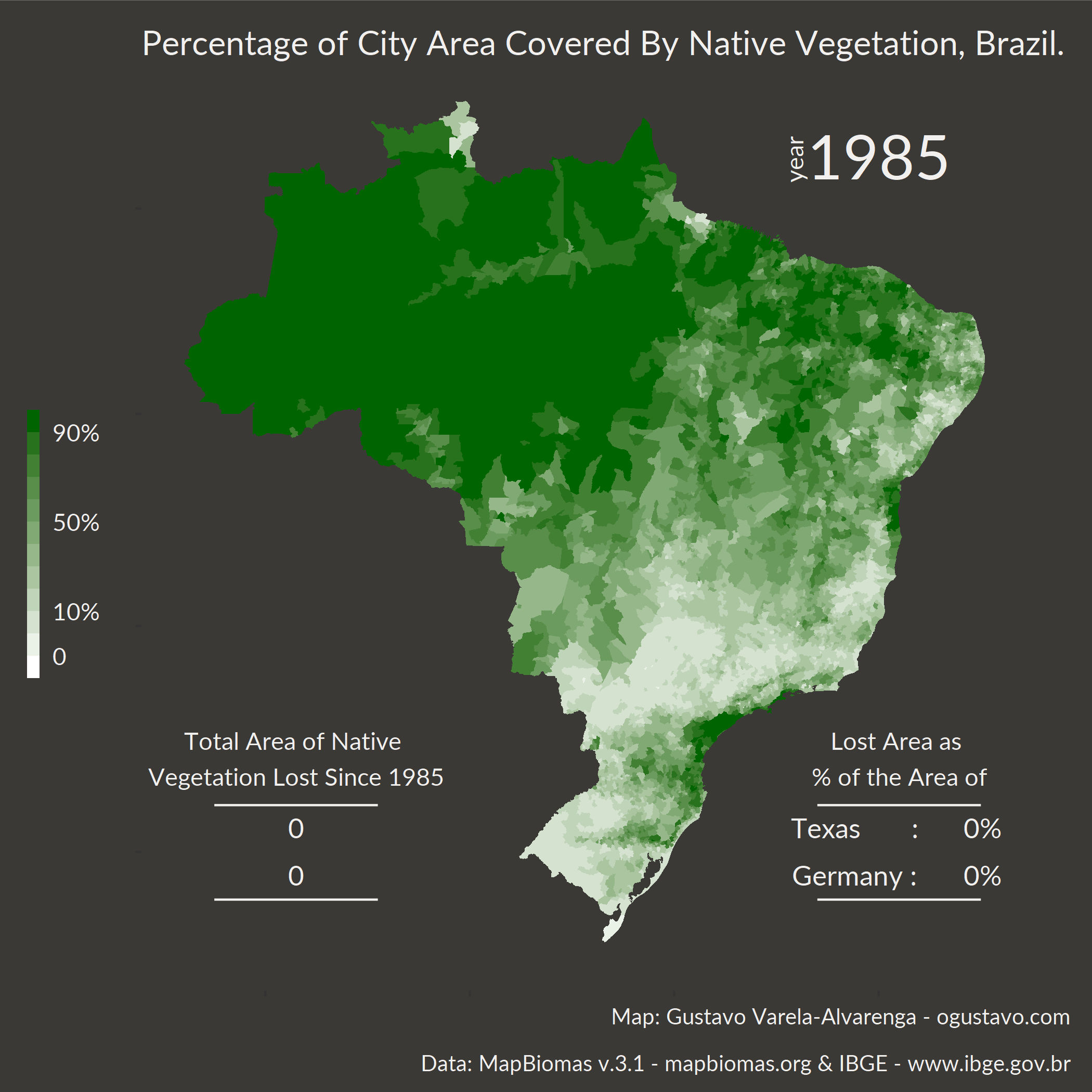
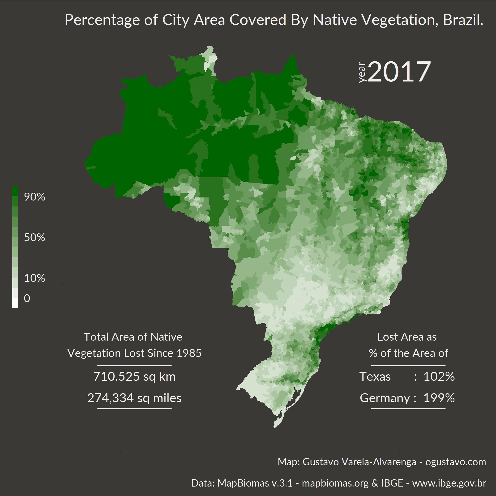
I wanted to focus on Natural Forest Formation data only and see how its total area evolved since 1985.
This tutorial has 3 sections, besides this introduction. The second section just goes over the packages and fonts that I used and how to download these fonts. In Section 3, I go over the data set and talk about its variables and their definitions. I also go over steps of importing the data set and doing some data manipulation to obtain the information that I want. Section 4 gives you the code for the final map.
You can download the .R file with the complete code from my GitHub.
Section 2: Packages
I’ll begin by going over the fonts I used and how to install them. I use Windows, so I don’t know if the same steps apply to other systems (sorry Mac and Unix users).
I’m using Lato, an open-source font family. So, make sure you download and install the Lato font before we start or you can just let R use the default system font - you won’t have to change the code, you will get some warning messages, but R will still plot the map.
You can download it from here.
The first thing I do is make sure that R can use this font, so I’ll use the extrafont package for that. If it’s your first time using these fonts you’ll have to run the font_import() command (this might take a while depending on the number of installed fonts you have, the good thing is that you’ll have to run this command only once).
# ************************************************************************* ----
# extrafont Package                                                         ----
# ************************************************************************* ----

#install.packages("extrafont")

library("extrafont")

# ************************************************************************* ----
# Import Font                                                               ----
# ************************************************************************* ----

# Install font Lato

# Run font_import only once:

# font_import()

# Check if Lato was imported
fonts()[grep("Lato", fonts())]
## [1] "Lato Black"    "Lato"          "Lato Hairline" "Lato Light"
## [5] "Lato Medium"   "Lato Thin"
# Register the fonts with R

loadfonts(device = "win")

# ************************************************************************* ----
# Remaining Packages                                                        ----
# ************************************************************************* ----

#install.packages("openxlsx")
#install.packages("tidyverse")
#install.packages("brazilmaps")
#install.packages("gifski")

library("openxlsx")
library("tidyverse")
library("brazilmaps")
library("gifski")
Section 3: The Data
Credit Where Credit is Due
The MapBiomas data are public, open and free through the simple reference of the source:
“Project MapBiomas - Collection 3.1 of Brazilian Land Cover & Use Map Series, accessed on 04/24/2019 through the link: (http://mapbiomas.org/pages/estatisticas")
“MapBiomas Project - is a multi-institutional initiative to generate annual land cover and use maps using automatic classification processes applied to satellite images. The complete description of the project can be found at http://mapbiomas.org“
I’m also using data on the area of the cities in Brazil from IBGE (the Brazilian Institute of Geography and Statistics). Due to changes in the size of the cities over the years, I’ve decided to use data from 2016. I was getting some incorrect results using data from 2017 or 2018, like cities with over 100% of their area covered by native vegetation. Clearly, these cities were divided but this wasn’t accounted for in MapBiomas’ data set. No cities with over 100% of their area covered by native vegetation were observed when using 2016 data.
The code below imports the data sets to R, but if you want you can download the xlsx files from the official sites by clicking here for MapBiomas’ data set and here for IBGE’s data set.
For the sake of maintaining my code, I’m also uploading the original databases to my GitHub repository and that’s the data I’ll use in my code below.
Data Dictionary
MapBiomas’ xlsx file has the following worksheet:
- INSTRUCTIONS;
- LAND COVER - BIOMAS e UF;
- LAND COVER - MUN_UF;
- CONSULTA BIOMA-UF; and
- CONSULTA MUN-UF.
I’ll use the LAND COVER - MUN_UF worksheet. The variables in this worksheet are:
| Variable | Class | Description |
|---|---|---|
| COD_ESTADO | numeric | state identifier |
| estado | character | state name |
| CODIBGE | numeric | city identifier |
| municipio | character | city name |
| cod.classe | numeric | land cover class identifier |
| nivel1 | character | class level 1 |
| nivel2 | character | class level 2 |
| nivel3 | character | class level 3 |
| 1985 | numeric | covered area in hectares(ha) in 1985 |
| … | … | … |
| 2017 | numeric | covered area in hectares(ha) in 2017 |
IBGE’s xlsx file has the following worksheet.
- AR_BR_MUN_2016;
- AR_BR_UF_2016;
- AR_BR_RG_2016; and
- AR_BR_2016.
I’ll use the AR_BR_MUN_2016 worksheet. The variables in this worksheet are:
| Variable | Class | Description |
|---|---|---|
| ID | numeric | ID |
| CD_GCUF | character | state identifier |
| NM_UF | character | state name |
| NM_UF_SIGLA | character | state abbreviation |
| CD_GCMUN | character | city identifier |
| NM_MUN_2016 | character | city name |
| AR_MUN_2016 | numeric | area in squared km |
I’m also creating the data set brazil.map with the shapefiles
to plot Brazil’s map divided by city using the function brazilmaps::get_brmap.
# ************************************************************************* ----
# Data Import                                                               ----
# ************************************************************************* ----
# Change number format
options(scipen=10)

# File Path on GitHub
file_path_forest_area = paste0(
  "https://github.com/gu-stat/forest-area/blob/master/",
  "data/Dados_Cobertura_MapBiomas_3.1_Biomas-UF-Municipios_%20SITE_UNPROTECTED.xlsx",
  "?raw=true")

file_path_city_area = paste0(
  "https://github.com/gu-stat/forest-area/blob/master/",
  "data/AR_BR_RG_UF_MUN_2016.xlsx",
  "?raw=true")

# Import
df.original <- openxlsx::read.xlsx(file_path_forest_area,
                                   sheet = "LAND COVER - MUN_UF")

df.city.area <- openxlsx::read.xlsx(file_path_city_area,
                                    sheet = "AR_BR_MUN_2016")

## \__ Map Data by City ----

brazil.map <- get_brmap(geo = "City", class = "sf")
Data Manipulation
# ************************************************************************* ----
# Data Manipulation                                                         ----
# ************************************************************************* ----

## \__ Transform City Code into Numeric ----

df.city.area2 <-
  df.city.area %>%
  dplyr::mutate(CODIBGE = as.numeric(CD_GCMUN)) %>%
  dplyr::select(CODIBGE, AR_MUN_2016)


## \__ Natural Forest Coverage Area Data ----

df.nat.forest <-
  df.original %>%
  filter(nivel2 == "Floresta Natural") %>%
  select(COD_ESTADO, estado, CODIBGE, nivel2, nivel3,
         paste0(seq(1985, 2017))
  ) %>%
  # SUM THE DIFFERENT SUB-GROUPS OF NATURAL FOREST
  group_by(COD_ESTADO, estado, CODIBGE) %>%
  summarize_at(vars(-nivel2,-nivel3),sum) %>%
  ungroup()

## \__ Join with City Area Data ----

df.nat.forest.AREA <-
  df.nat.forest %>%
  # ADD TOTAL AREA OF MUNICIPALITY TO DATA SET
  dplyr::left_join(x = ., y = df.city.area2, by = "CODIBGE") %>%
  # CREATE PERCENTAGES
  ## Divide x/100 to transform from hectares to squared km
  dplyr::mutate_at(.vars=vars(paste0(seq(1985,2017))),
                   .fun = function(x) round(100*((x/100)/.$AR_MUN_2016),3)
  )


# CHECK IF ANYTHING GREATER THAN 100%
greater.1 <- NULL
for (i in 1985:2017) {
  greater.1 <- append(greater.1, which(df.nat.forest.AREA[,paste0(i)] >= 100))
}

greater.1 <- greater.1 %>% unlist() %>% unique()

## \__ Create Percentages Breaks ----

df.nat.forest.AREA <-
  df.nat.forest.AREA %>%
  dplyr::mutate_at(.vars=vars(paste0(seq(1985,2017))),
                   .fun = function(x) cut(x,breaks=c(-Inf, 0, 1, seq(0, 100, 10)[-1]))
  )
Section 4: The Map
# ************************************************************************* ----
# Map                                                                       ----
# ************************************************************************* ----

## \__ Function that Joins Map Data by City with Forest Area Data ----

create.map.df <- function(DATA){

  map <- join_data(map = brazil.map, data = DATA, by = c("City" = "CODIBGE"))

  map.ggplot <- as(map, "Spatial")

  map.ggplot@data$id = row.names(map.ggplot@data)

  df.map.ggplot <- suppressMessages(ggplot2::fortify(map.ggplot))

  df.map.ggplot <- dplyr::left_join(df.map.ggplot, map.ggplot@data, by = "id")

  return(df.map.ggplot)
}

## \____ Map Data for Plot ----

df.map.ggplot <- create.map.df(df.nat.forest.AREA)

## \__ Map Colors ----

# USE https://gka.github.io/palettes TO GET
# COLOR SCALE FROM white TO darkgreen
# THAT'S ALSO SUITABLE TO COLORBLIND PEOPLE WITH 12 BREAKS
# SAME NUMBER AS THE LEVELS OF cut(x,breaks=c(-Inf, 0, 1, seq(0, 100, 10)[-1]))

map.colors <- c('#ffffff','#eaf1e7','#d4e2cf','#bfd4b8','#abc5a1','#96b78a',
                '#81a974','#6c9b5f','#588d4a','#428034','#28711d','#006400')

### \__ Map Labels ----

map.labels <- c("0", "", "10%", rep("",3), "50%", rep("",3), "90%", "")

## \__ Create Theme ----

map.theme <-
  theme(
    text = element_text(size = 13, family = "Lato", color = "#f2efef"),
    axis.text = element_blank(),
    axis.title.x = element_blank(),
    axis.title.y = element_blank(),
    plot.background = element_rect(fill = "#3a3935", color = NA),
    panel.background = element_rect(fill = "#3a3935", color = NA),
    panel.grid = element_blank(),
    plot.margin = margin(t = 0.25,r = 0.25,b = 0.25,l = 0.25,unit = "cm"),
    plot.title = element_text(margin = margin(t = 0.25, unit = "cm")),
    plot.caption = element_text(size = 10),
    legend.background = element_rect(fill = "#3a3935", color = "#3a3935"),
    legend.text = element_text(size = 11),
    legend.title = element_text(size = 12),
    legend.position = "left",
    legend.key = element_rect(color = "transparent"),
    legend.key.size = unit(0, units = "mm"),
    legend.key.width = unit(2, units = "mm")
  )

## \__ Plot Map ----

### \____ Function for GIF ----
plot.map.forest <- function(){
  for (i in 1985:2017) {

    lost.area.year.km2 <-
      round(
        sum(-(df.nat.forest %>% summarize_at(paste0(i),sum)/100),
            df.nat.forest %>% summarize_at(paste0(1985),sum)/100)
        ,2
      )

    lost.area.year.mi2 <- round(lost.area.year.km2/2.59, 2)

    map.forest <-
      # MAP
      ggplot(mapping = aes(x = long, y = lat, group = group)) +
      # MAP WITH TRANSPARENT CITY LINES
      geom_polygon(
        data = df.map.ggplot,
        aes_string(fill = paste0("X",i)),
        color = "transparent"
      ) +
      # LEGEND
      scale_fill_manual(
        values = map.colors,
        drop = FALSE,
        na.value = "black",
        na.translate = FALSE,
        name = "",
        label = map.labels,
        guide = guide_legend(
          direction = "vertical",
          ncol = 1,
          reverse = TRUE,
          label.vjust = 2.5
        )
      ) +
      # MAP LIMITS
      xlim(range(df.map.ggplot$long)) +
      ylim(range(df.map.ggplot$lat)) +
      coord_map() +
      # ADD TITLE AND CAPTIONS
      labs(
        title = "Percentage of City Area Covered By Native Vegetation, Brazil.",
        caption = paste0("Map: Gustavo Varela-Alvarenga - ogustavo.com \n \n ",
                         "Data: MapBiomas v.3.1 - mapbiomas.org & ",
                         "IBGE - www.ibge.gov.br ")
      ) +
      # ADD THEME
      map.theme +
      # ADD ANNOTATIONS
      ## WORD YEAR
      annotate(
        geom = "text", x = -44.1, y = 2.4, size = 4, family = "Lato",
        color = "#f2efef", label = "year", angle = 90
      ) +
      ## ACTUAL YEAR
      annotate(
        geom = "text", x = -40, y = 2.5, size = 10, family = "Lato",
        color = "#f2efef", label = paste0(i)
      ) +
      ## TITLE - TABLE ON THE LEFT
      annotate(
        geom = "text", x = -68.5, y = -26, size = 4, family = "Lato",
        color = "#f2efef", hjust = 0.5,
        label =
          paste0("Total Area of Native \n", "Vegetation Lost Since 1985")
      ) +
      ## LINE BELOW TITLE
      annotate(
        geom = "segment", x = -64.5, xend = -72.5, y = -28, yend = -28,
        linetype = "solid", color = "#f2efef"
      ) +
      ## VALUES IN KM2 WITH . TO MARK THOUSANDS
      annotate(
        geom = "text", x = -68.5, y = -29, size = 4.5, family = "Lato",
        color = "#f2efef", hjust = 0.5,
        label =
          ifelse(lost.area.year.km2 == 0, "0",
                 paste0(prettyNum(round(lost.area.year.km2, 0),
                                  big.mark=".", decimal.mark = ","),
                        " sq km")
          )
      ) +
      ## VALUES IN MI2 WITH , TO MARK THOUSANDS
      annotate(
        geom = "text", x = -68.5, y = -31, size = 4.5, family = "Lato",
        color = "#f2efef", hjust = 0.5,
        label =
          ifelse(lost.area.year.mi2 == 0, "0",
                 paste0(prettyNum(round(lost.area.year.mi2, 0), big.mark=","),
                        " sq miles")
          )
      ) +
      ## LINE BELOW TABLE
      annotate(
        geom = "segment", x = -64.5, xend = -72.5, y = -32, yend = -32,
        linetype = "solid", color = "#f2efef"
      ) +
      ## TITLE - TABLE ON THE RIGHT
      annotate(
        geom = "text", x = -39, y = -26, size = 4, family = "Lato",
        color = "#f2efef", hjust = 0.5,
        label =  paste0("Lost Area as \n", "% of the Area of")
      ) +
      ## LINE BELOW TITLE
      annotate(
        geom = "segment", x = -35, xend = -43, y = -28, yend = -28,
        linetype = "solid", color = "#f2efef"
      ) +
      ## ADD WORD TEXAS
      annotate(
        geom = "text", x = -41, y = -29, size = 4.5, family = "Lato",
        color = "#f2efef", label =  "Texas       : "
      ) +
      ## ADD VALUE FOR TEXAS
      annotate(
        geom = "text", x = -34, y = -29, size = 4.5, family = "Lato",
        color = "#f2efef", hjust = 1,
        label =
          ifelse(
            lost.area.year.km2 == 0, "0%",
            paste0(round(lost.area.year.km2/696241, 2) * 100, "%")
          )
      ) +
      ## ADD WORD GERMANY
      annotate(
        geom = "text", x = -41, y = -31, size = 4.5, family = "Lato",
        color = "#f2efef", label =  "Germany : "
      ) +
      ## ADD VALUE FOR GERMANY
      annotate(
        geom = "text", x = -34, y = -31, size = 4.5, family = "Lato",
        color = "#f2efef", hjust = 1,
        label =
          ifelse(
            lost.area.year.km2 == 0, "0%",
            paste0(round(lost.area.year.km2/357386, 2) * 100, "%")
          )
      ) +
      ## LINE BELOW TABLE
      annotate(
        geom = "segment", x = -35, xend = -43, y = -32, yend = -32,
        linetype = "solid", color = "#f2efef"
      )

    print(map.forest)

  }
}
### \____ Create GIF ----
### Be mindful that this will save a gif file named forest_animation.gif into
### your working directory

gif_file <-
  gifski::save_gif(
    expr = plot.map.forest(),
    gif_file = "forest_animation.gif",
    delay = 0.75, width = 738, height = 788, res = 100
  )

utils::browseURL(gif_file)
If you want you can you use the code below to get high-quality static images of the maps. Be mindful that this will save the plots into your working directory.
#install.packages("Cairo")
library("Cairo")

for (i in 1985:2017) {

    lost.area.year.km2 <-
      round(
        sum(-(df.nat.forest %>% summarize_at(paste0(i),sum)/100),
            df.nat.forest %>% summarize_at(paste0(1985),sum)/100)
        ,2
      )

    lost.area.year.mi2 <- round(lost.area.year.km2/2.59, 2)

    map.forest <-
      # MAP
      ggplot(mapping = aes(x = long, y = lat, group = group)) +
      # MAP WITH TRANSPARENT CITY LINES
      geom_polygon(
        data = df.map.ggplot,
        aes_string(fill = paste0("X",i)),
        color = "transparent"
      ) +
      # LEGEND
      scale_fill_manual(
        values = map.colors,
        drop = FALSE,
        na.value = "black",
        na.translate = FALSE,
        name = "",
        label = map.labels,
        guide = guide_legend(
          direction = "vertical",
          ncol = 1,
          reverse = TRUE,
          label.vjust = 2.5
        )
      ) +
      # MAP LIMITS
      xlim(range(df.map.ggplot$long)) +
      ylim(range(df.map.ggplot$lat)) +
      coord_map() +
      # ADD TITLE AND CAPTIONS
      labs(
        title = "Percentage of City Area Covered By Native Vegetation, Brazil.",
        caption = paste0("Map: Gustavo Varela-Alvarenga - ogustavo.com \n \n ",
                         "Data: MapBiomas v.3.1 - mapbiomas.org & ",
                         "IBGE - www.ibge.gov.br ")
      ) +
      # ADD THEME
      map.theme +
      # ADD ANNOTATIONS
      ## WORD YEAR
      annotate(
        geom = "text", x = -44.1, y = 2.4, size = 4, family = "Lato",
        color = "#f2efef", label = "year", angle = 90
      ) +
      ## ACTUAL YEAR
      annotate(
        geom = "text", x = -40, y = 2.5, size = 10, family = "Lato",
        color = "#f2efef", label = paste0(i)
      ) +
      ## TITLE - TABLE ON THE LEFT
      annotate(
        geom = "text", x = -68.5, y = -26, size = 4, family = "Lato",
        color = "#f2efef", hjust = 0.5,
        label =
          paste0("Total Area of Native \n", "Vegetation Lost Since 1985")
      ) +
      ## LINE BELOW TITLE
      annotate(
        geom = "segment", x = -64.5, xend = -72.5, y = -28, yend = -28,
        linetype = "solid", color = "#f2efef"
      ) +
      ## VALUES IN KM2 WITH . TO MARK THOUSANDS
      annotate(
        geom = "text", x = -68.5, y = -29, size = 4.5, family = "Lato",
        color = "#f2efef", hjust = 0.5,
        label =
          ifelse(lost.area.year.km2 == 0, "0",
                 paste0(prettyNum(round(lost.area.year.km2, 0),
                                  big.mark=".", decimal.mark = ","),
                        " sq km")
          )
      ) +
      ## VALUES IN MI2 WITH , TO MARK THOUSANDS
      annotate(
        geom = "text", x = -68.5, y = -31, size = 4.5, family = "Lato",
        color = "#f2efef", hjust = 0.5,
        label =
          ifelse(lost.area.year.mi2 == 0, "0",
                 paste0(prettyNum(round(lost.area.year.mi2, 0), big.mark=","),
                        " sq miles")
          )
      ) +
      ## LINE BELOW TABLE
      annotate(
        geom = "segment", x = -64.5, xend = -72.5, y = -32, yend = -32,
        linetype = "solid", color = "#f2efef"
      ) +
      ## TITLE - TABLE ON THE RIGHT
      annotate(
        geom = "text", x = -39, y = -26, size = 4, family = "Lato",
        color = "#f2efef", hjust = 0.5,
        label =  paste0("Lost Area as \n", "% of the Area of")
      ) +
      ## LINE BELOW TITLE
      annotate(
        geom = "segment", x = -35, xend = -43, y = -28, yend = -28,
        linetype = "solid", color = "#f2efef"
      ) +
      ## ADD WORD TEXAS
      annotate(
        geom = "text", x = -41, y = -29, size = 4.5, family = "Lato",
        color = "#f2efef", label =  "Texas       : "
      ) +
      ## ADD VALUE FOR TEXAS
      annotate(
        geom = "text", x = -34, y = -29, size = 4.5, family = "Lato",
        color = "#f2efef", hjust = 1,
        label =
          ifelse(
            lost.area.year.km2 == 0, "0%",
            paste0(round(lost.area.year.km2/696241, 2) * 100, "%")
          )
      ) +
      ## ADD WORD GERMANY
      annotate(
        geom = "text", x = -41, y = -31, size = 4.5, family = "Lato",
        color = "#f2efef", label =  "Germany : "
      ) +
      ## ADD VALUE FOR GERMANY
      annotate(
        geom = "text", x = -34, y = -31, size = 4.5, family = "Lato",
        color = "#f2efef", hjust = 1,
        label =
          ifelse(
            lost.area.year.km2 == 0, "0%",
            paste0(round(lost.area.year.km2/357386, 2) * 100, "%")
          )
      ) +
      ## LINE BELOW TABLE
      annotate(
        geom = "segment", x = -35, xend = -43, y = -32, yend = -32,
        linetype = "solid", color = "#f2efef"
      )

    ### Be mindful that this will save several png files named Y*.png,
    ### where * is the year, into your working directory

    ggsave(
      paste0("Y",i,".png"), device="png", type="cairo",
      width = 7, height = 7
    )

  }